Tokens Aren't Dying. They're Ceding the Middle.
Three verdicts: information theory, information geometry, representation theory.
BLUF
The claim: tokens don’t die. They cede the latent middle.
Three independent mathematical tools, three independent verdicts on discrete tokens versus continuous embeddings:
- Information theory — a draw. Both inherit the same source-coding loss. Shannon does not permit a free lunch.
- Information geometry — continuous wins. The Fisher matrix is singular at the simplex boundary; Wasserstein-2 space is smooth. This is the mathematical root of the training-efficiency results in ELF and Cola DLM.
- Representation theory — the field splits. The physical world carries Lie group structure (SO(3), Galilean) that continuous embeddings can honour. Language carries free-monoid compositional structure, and a discrete token is the equivalence class.
Combined, they point at one concrete architecture: discrete at the IO boundary, continuous through the latent middle, training signal extended beyond language.
“Tokens must die” is rhetoric. “Tokens cede the latent middle” is the mathematical verdict.
I. When the argument became quantifiable
In the first half of 2026, two engineering results turned a long-running philosophical argument into numbers.
Kaiming He’s team published ELF (Embedded Language Flows), which keeps the whole of text generation inside a continuous vector space and only projects back to human-readable text at the final step. Thirty-two sampling steps, generation quality above what discrete models produce in 1024, trained on roughly 45 billion tokens — about a tenth of what mainstream approaches use. Four days later ByteDance Seed released Cola DLM, which uses a Text VAE to compress language into a deeper semantic latent space, models the global prior there with flow matching, and only then decodes back to text.
Two papers, at moderate scale, showing the same counterintuitive shape: fewer sampling steps, less training data, higher quality.
What’s interesting isn’t which paradigm won. It’s that this drags “language is a lossy compression protocol” — a claim that had been sitting at the philosophical level — down onto quantifiable engineering metrics. Once an argument becomes quantifiable, mathematics gets a vote.
So: a structural audit of the token paradigm using three tools — information theory, information geometry, representation theory. Each is independent. Each returns its own verdict. Only the three together represent what mathematics actually has to say about the fate of tokens.
Spoiler: tokens have no information-theoretic disadvantage of their own, they do have a quantifiable geometric disadvantage in the latent middle, and the IO boundary plus linguistic compositionality gives them a position nothing else fills. The three together point not at death but at fusion — and at a specific shape for the next architecture.
II. Layer one: information theory
Shannon’s 1948 source coding theorem gives a hard bound: for any random variable X, lossless compression cannot average fewer bits than its entropy H(X). Lossy compression is bounded by the rate-distortion function R(D) — given tolerable distortion D, the minimum rate is R(D).
Applied to training large models, the signal path looks like this:
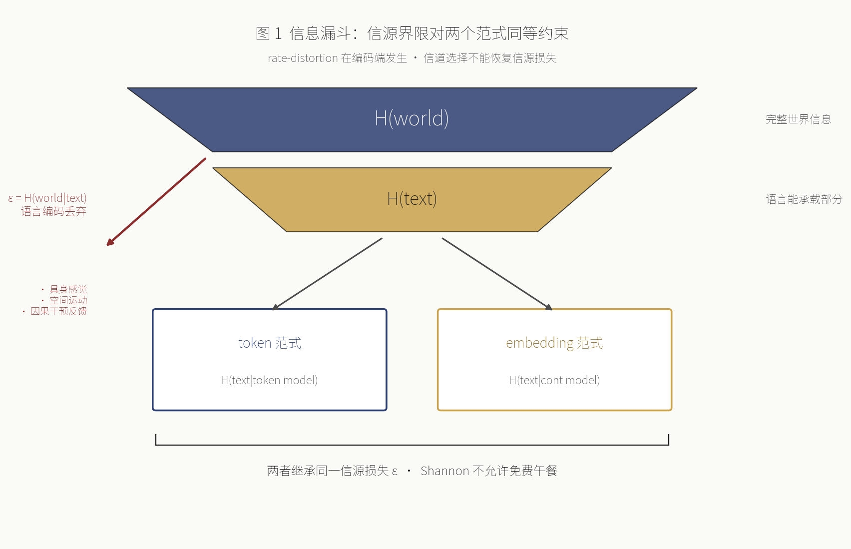
What a model can learn about the world from a corpus is bounded above by H(world) − H(world | text). That second term is what remains uncertain about the world after you have all the text — that is, the world-structure discarded by the human language encoding process. And that discarding happens at the encoder. The embodied sensation of pain, the muscle memory of moving through space, the physical feedback of causal intervention: almost none of it was ever written down in any human language.
This is the layer LeCun keeps pointing at. At the information-theoretic level, he’s right.
But the next inferential step skips a beat: tokens are the product of this lossy encoding, therefore the token paradigm cannot reach the discarded dimensions. The problem is that continuous embeddings are equally a product of that encoding. ELF finishes generation in ℝᵈ; Cola DLM compresses to a deep latent via Text VAE and flow-matches there. The training signal for both still originates in human-produced text. Changing the channel format does not recover information lost at the source. Shannon does not permit that free lunch.
Put differently: if information theory were the deciding criterion, tokens and continuous embeddings should be condemned together, not one of them carried out on shoulders. For either to recover the discarded dimensions, the training signal has to be extended into non-linguistic channels — embodied interaction, physics simulation, object dynamics in video, robot sensor streams. That is what the JEPA line and the SSI line are actually betting on, and it is a different bet from swapping tokens for embeddings.
Verdict, layer one: a draw. Mistaking a source bound for a channel-selection problem is a category error.
III. Layer two: information geometry
If layer one is a draw, where do the paradigms actually separate? In optimisation geometry.
Amari’s information geometry, developed through the 1980s, says a neural network’s parameter space is not Euclidean but a Riemannian manifold carrying the Fisher information metric. The distance between two parameter points should be measured by the KL divergence between the distributions they induce, not by Euclidean difference in parameters. That metric determines the true geometry of gradient descent — the natural gradient corrects direction using the inverse Fisher matrix and is the statistically optimal update.
Apply it to both paradigms. The core difference lies in the manifold their output distributions live on:
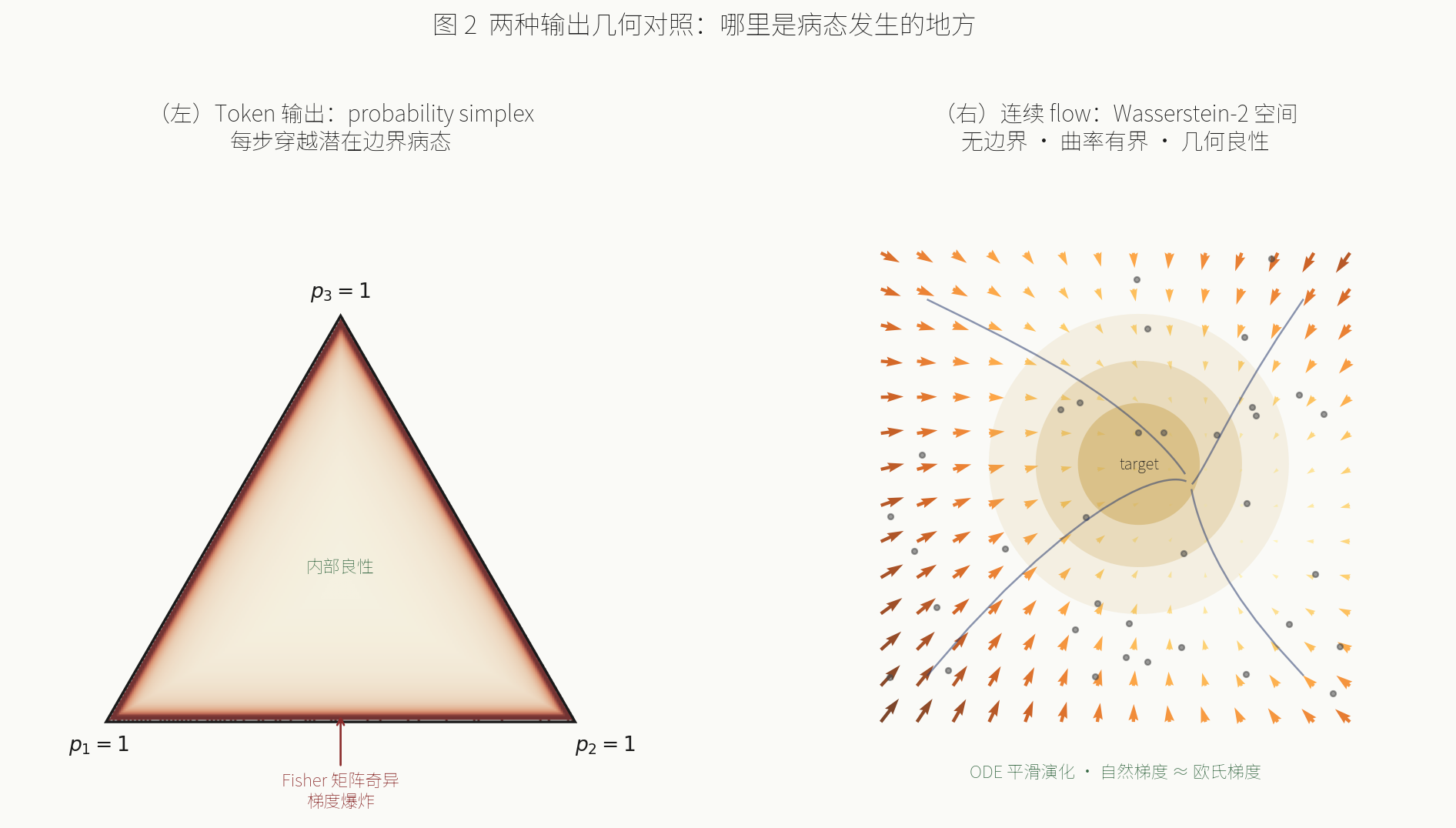
Token autoregression. At each timestep the model emits a categorical distribution p(xₜ | x₍₌ₜ), valued on the |V|-dimensional probability simplex. That simplex has poor geometry. The boundary is degenerate — some coordinates go to zero — and near the boundary the Fisher matrix becomes singular, gradient directions blow up, and the optimisation path has to steer clear. In practice, label smoothing pushes the distribution away from the boundary and temperature scaling tunes sharpness. Both are, at bottom, workarounds for simplex boundary pathology.
Continuous flow matching. The model learns a velocity field v_θ(x, t) on ℝᵈ, pushing a noise distribution to the target embedding distribution via an ODE. The whole optimisation happens in Wasserstein-2 space, where probability measures are compared by optimal transport distance. That space has no boundary, bounded curvature, a smooth Riemannian metric, and a natural gradient that approximates the Euclidean one. The optimisation geometry is benign.
This is the mathematical root of ELF beating a discrete model’s 1024 steps in 32, on a tenth of the data. It isn’t that the network is cleverer. It’s that it optimises in Wasserstein space, whose geometry is friendlier than the simplex. Cola DLM’s extra Text VAE layer, compressing to a deeper semantic latent, is essentially removing the simplex’s discrete symptoms from the core modelling process entirely.
But there’s a detail both papers step around: however elegant the latent, the final step still has to decode back to tokens. That step is a latent → categorical projection, and the geometric pathology returns. The difference is where it occurs. The token path absorbs simplex pathology at every timestep — accumulated 1024 times. The continuous path absorbs it once, at the end. More economical, but not eliminated.
Verdict, layer two: in the latent middle, tokens lose to continuous embeddings, and on optimisation geometry there is no path back. This is the real engineering signal ELF and Cola DLM contribute, and the physical motivation for fusion architectures. The discrete projection at the IO boundary remains unavoidable.
IV. Layer three: representation theory
The third verdict is the subtlest, and the one the “tokens must die” narrative most reliably ignores.
Representation theory — and its incarnation in deep learning, group-equivariant neural networks — answers one question: what symmetry structure does a given kind of data naturally carry, and which architectures can honour it?
Formally: if a group G acts on data x, the ideal model φ should satisfy φ(g · x) = g · φ(x), i.e. be G-equivariant. Cohen and Welling reorganised CNNs group-theoretically in 2016 — translation equivariance is the action of ℤ², rotation extends to SO(2), 3D rotation to SO(3).
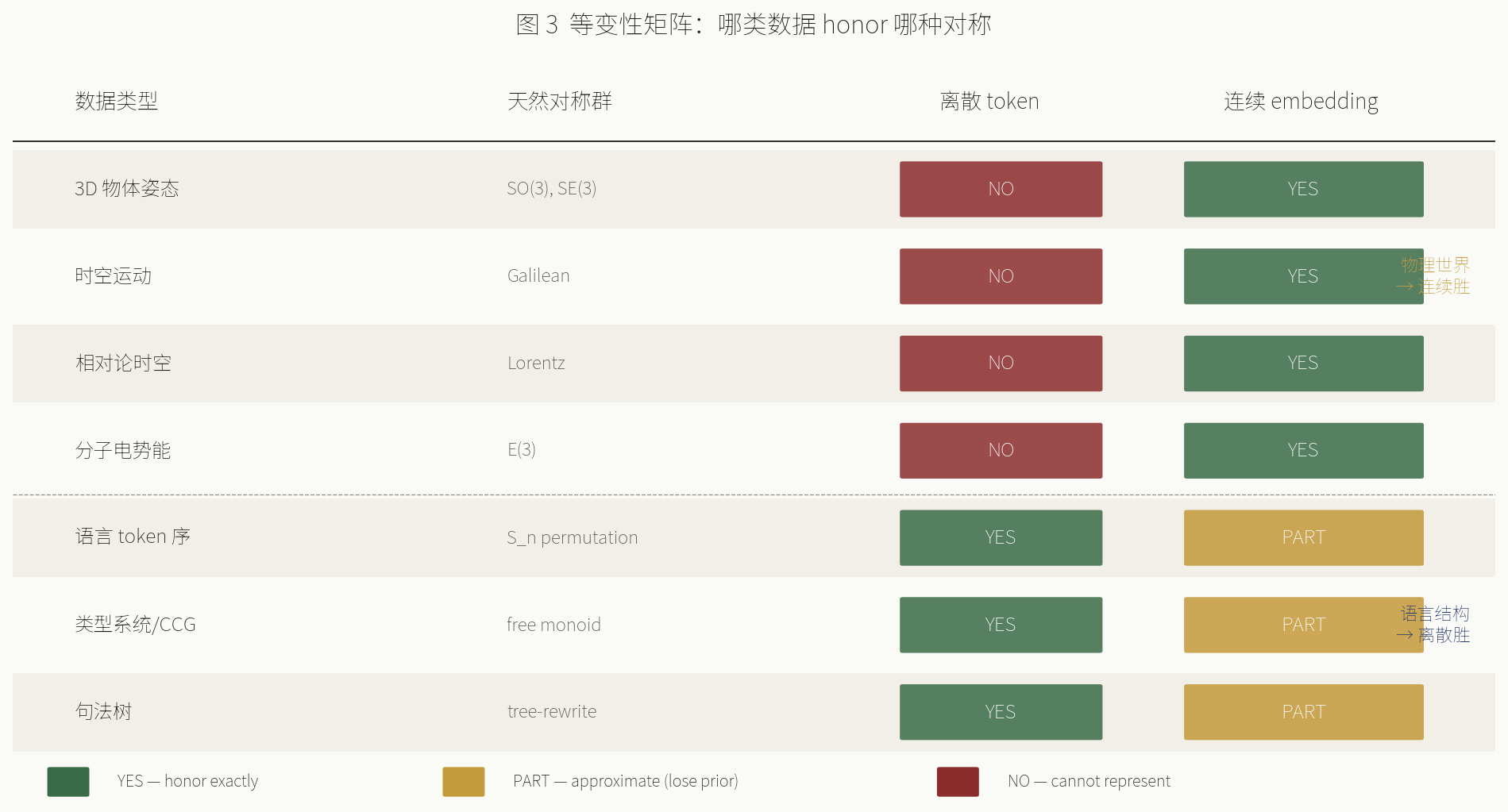
On the physical world, mathematics stands with the continuous side. The physical world natively carries Lie group structure: SE(3) for rigid-body motion, Galilean for classical spacetime, Lorentz for relativistic. A molecule’s electrostatic potential energy doesn’t depend on how you rotate it. A robot grasp’s success rate doesn’t depend on shifting the camera half a metre left. These are continuous Lie groups, and a continuous embedding space can carry their action directly — you can design SO(3)-equivariant layers on ℝᵈ such that rotating the input rotates the intermediate representation in step. The JEPA line, the masked-autoencoder lineage, and essentially all frontier work in 3D vision and robot control rest on this. Token sequences carry no continuous Lie group action; the most you have is a discrete permutation group Sₙ, which cannot capture SO(3) equivariance.
This is the underlying justification for continued betting on the world-model line, and why embodied intelligence cannot stay on a token-only architecture.
But the same representation theory delivers a verdict for the other side.
Language’s structure is compositional structure on a free monoid — words compose into phrases, phrases into sentences, carrying a type system (Montague semantics, typed lambda calculus, CCG). These are discrete objects with discrete group structure: free generators on a syntax tree. Force that into a continuous embedding in ℝᵈ and you can approximate the structure, but approximation is not exactness. The same “the cat sat on the mat” has infinitely many neighbouring representations in continuous space, and the model has to spend capacity approximating that equivalence class — whereas a discrete token simply is the equivalence class.
Which is why purely continuous language models keep losing to hybrids that retain discrete tokens on compositional generalisation tasks — Lake and Baroni’s SCAN benchmark series, and several comparative studies on compositional skills. Language’s compositional prior is carried by the discrete objects themselves. Throw away the tokens and you throw away the prior, and the model has to rebuild it with more capacity and more data.
Verdict, layer three: split. Physical perception and world modelling → continuous. Linguistic compositionality → discrete wins or ties. This layer cannot be flattened into “continuous sweeps.”
The counterargument: tokenizer-free and byte-level models
Honestly stated, this section has a counterargument that deserves to be taken seriously: discrete IO isn’t a prior, it’s historical baggage.
Byte-level Transformers, CANINE, ByT5, and recent byte-level Mamba variants all try to route around the traditional tokenizer and model the byte stream directly. The implicit claim is that language’s compositional structure need not be handed to the model explicitly by a tokenizer — the model can learn it from bytes. If that holds at frontier scale, §IV’s argument that discrete tokens are an indispensable prior needs re-examination. Though note that what you’d have is byte-level discrete units rather than BPE subwords — still discrete IO.
A more aggressive version goes further: bytes are also an arbitrary convention (UTF-8 is an encoding, not a natural unit), so why not model the continuous signal directly? That route currently works only in audio — WaveNet, SoundStream, Encodec — with no frontier-scale instance for text.
The position here: the discrete IO boundary almost certainly survives, but the granularity of that discreteness is open. BPE tokens, bytes, characters all fall under “discrete.” The real source of the compositional prior is the equivalence-class structure discrete objects possess, not BPE as a specific engineering implementation. So layer three’s “language → discrete” verdict holds in the abstract, while which discrete representation wins will be settled by engineering experiment over the next 24 months. Falsifier F2 below is the concrete indicator to watch.
V. Combining the three
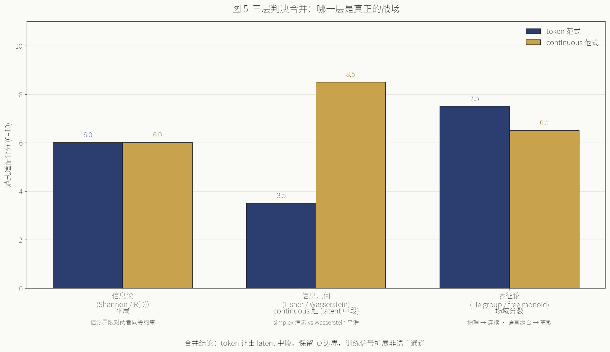
| Layer | Tool | Tokens | Continuous | Verdict |
|---|---|---|---|---|
| Information theory | Shannon, rate-distortion | bounded by the source | equally bounded | draw |
| Information geometry | Amari, Fisher metric, Wasserstein | simplex pathology | Wasserstein benign | continuous wins (latent middle) |
| Representation theory | Lie group equivariance / free monoid | weak on physics, strong on language | strong on physics, weak on language | field splits |
Combined, the mathematics does not point at “tokens must die.” It points at a specific architectural shape:
- Keep discrete tokens at the IO boundary. The discrete prior on linguistic compositionality and the human-facing output format are both non-disposable. (Granularity may fall back from BPE to bytes or characters — see the counterargument above.)
- Move the latent middle to continuous. Wasserstein optimisation geometry and physical equivariance are both on the continuous side.
- Extend the training signal into non-linguistic channels. This is the only route to recovering the discarded dimensions, and it is orthogonal to the discrete/continuous choice.
Each of those three has independent mathematical justification. None of them needs a triumphalist narrative about one paradigm to hold them together. The real defect in the popular story is that it takes layer two’s local verdict — about the optimisation geometry of latent computation — and inflates it into a verdict across all three.
VI. Predicted evolution
Let t be relative time, with t=0 at 2026 Q2.
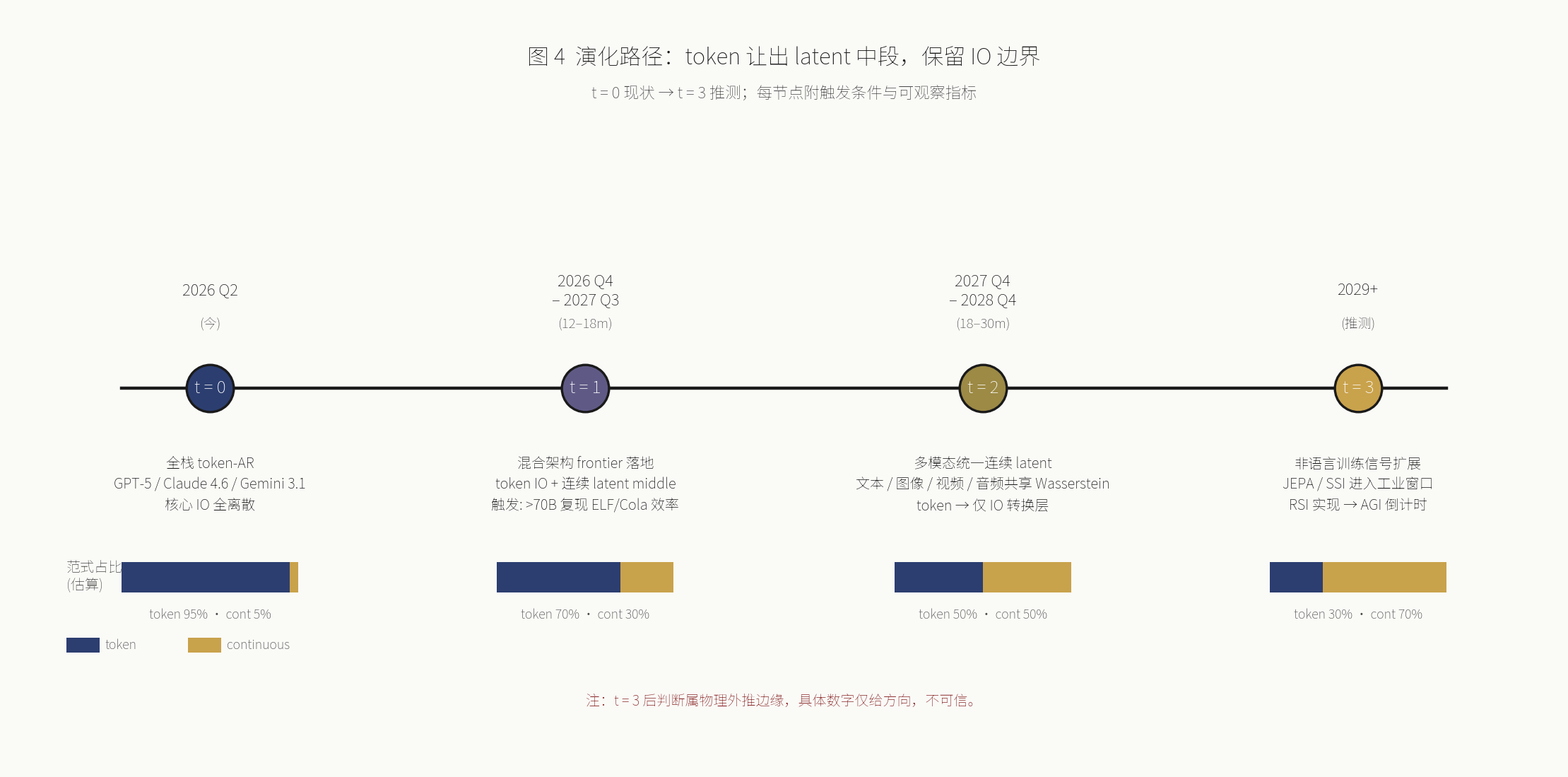
t=0, now (2026 Q2). Mainstream products are full-stack token-AR. Continuous latents appear only in multimodal encoders, TTS, and diffusion image generation. Industrial IO is entirely discrete tokens.
t=1 (est. 2026 Q4 – 2027 Q3, 12–18 months). Hybrid architectures reach frontier deployment in the text generation layer: token IO retained, core generation done in a continuous latent by flow matching or score-based diffusion. Trigger: some frontier lab reproduces ELF/Cola DLM training-efficiency advantages above 70B parameters with acceptable inference latency. Industrial marker: a 2–3× step change in inference throughput and training FLOP efficiency.
t=2 (est. 2027 Q4 – 2028 Q4, 18–30 months). Multimodal training happens in a unified continuous latent, with text, image, video, and audio sharing a Wasserstein space. Natively multimodal architectures become mainstream; others follow or get dragged down by technical debt. Tokens degrade into an input/output conversion layer and stop participating in core reasoning. Industrial marker: “multimodal capability” stops being a differentiator and becomes the default.
t=3 (est. post-2029, highly speculative). Training signal extends into non-linguistic channels — embodied interaction, physics simulation, self-evolving data. The JEPA and SSI lines enter their industrial validation window. If recursive self-improvement gets engineered in this period, the AGI timeline genuinely starts counting down. If not, the data wall and compute wall together push the frontier into saturation.
Anything past t=3 is at the edge of physical extrapolation. No specific number there is credible; only the direction is.
VII. Falsification dashboard
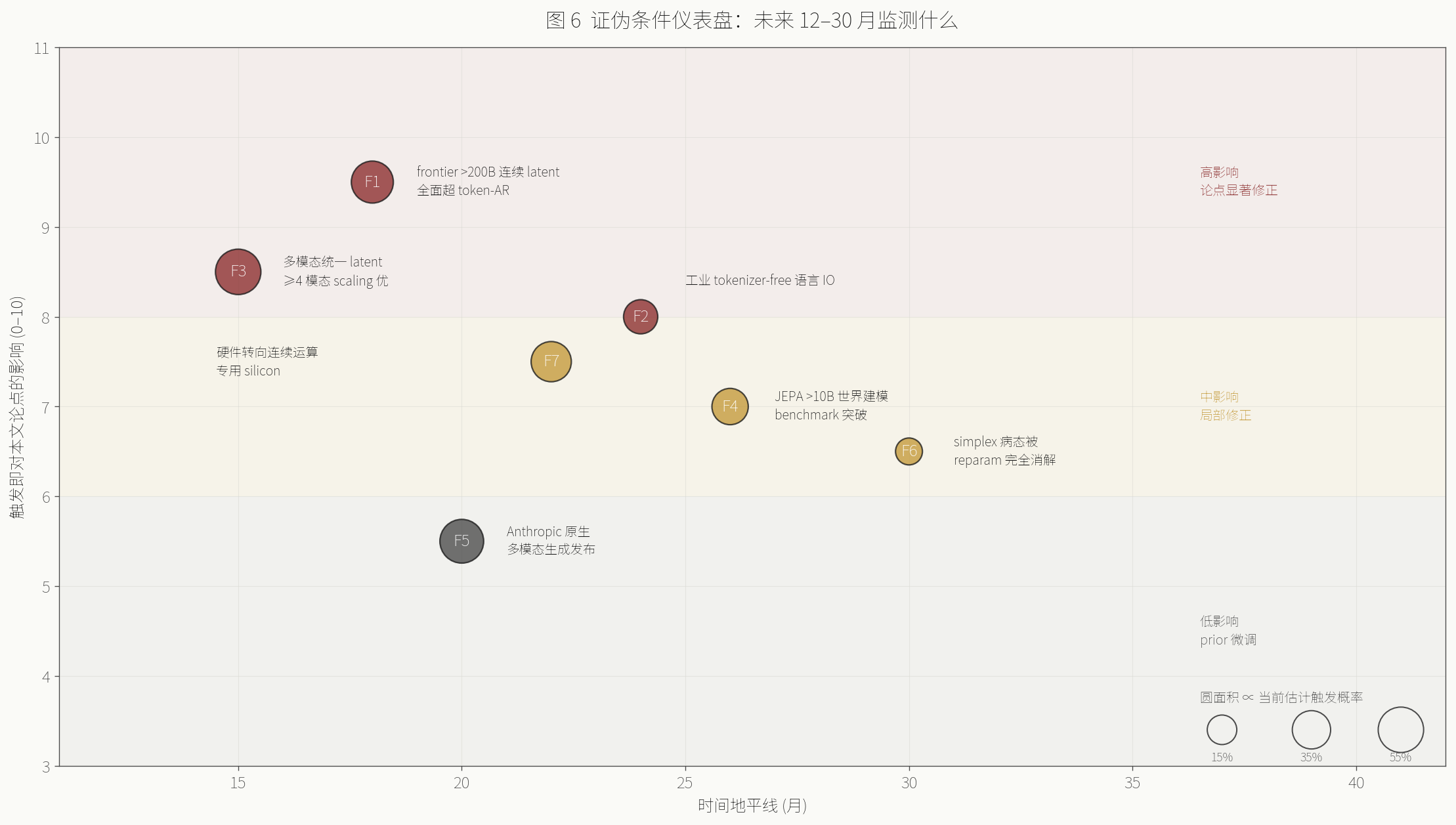
| # | Indicator | Direction of revision if triggered |
|---|---|---|
| F1 | Any frontier lab (>200B params) ships a continuous-latent model that beats token-AR across benchmarks at equal compute | Layer two strengthens; accelerate t=1 → t=2 |
| F2 | An industrial product ships a genuinely tokenizer-free language IO | Half of layer three overturned; the discrete-prior assumption needs re-examination |
| F3 | A unified continuous-latent multimodal model shows scaling laws across 4+ modalities with a better slope than the token paradigm | Pull t=2 forward by 12 months |
| F4 | The JEPA line produces no world-modelling benchmark breakthrough above 10B within two years | Push t=3 back |
| F5 | A proof that simplex geometric pathology is fully removable by a new reparameterisation | Layer two overturned; token-AR becomes competitive again in the latent layer |
| F6 | Compute supply chains visibly pivot toward continuous-operation optimisation (dedicated silicon for flow matching / score-based models) | Industry concedes the paradigm shift; accelerate t=1 → t=2 |
Zero triggers in a year and the prior holds. Two or more and this section needs rewriting.
VIII. Mathematics gives constraints, not answers
Can you deduce the future of tokens from mathematical logic?
No. Mathematics does not deduce technology timelines. What it gives you is structural constraints: certain things are impossible at certain layers, certain things are locally optimal at certain layers. Collect the constraints and you get a map of the permitted evolution space, not a specific trajectory through it.
“Tokens must die” is rhetoric, not a verdict. It works at the level of propagation and is irrelevant at the level of engineering. What will actually happen is that tokens cede the latent middle, keep the IO boundary, and the training signal extends into non-linguistic channels. Those three hold independently in mathematics and together constitute the shape of the next architecture.
Whether that shape leads to AGI is a separate question — and information theory says that as long as the training signal’s source is unchanged, no paradigm gets there. That is what the world-model line and the recursive-self-improvement line both see, and it’s why what they’re actually betting on isn’t continuous versus discrete. It’s active exploration versus passive imitation. That deserves its own piece.
Confidence: the mathematical results cited (Shannon source coding, Amari’s information geometry, Fisher singularity at the simplex boundary, Wasserstein-2 regularity, group equivariance) are settled (high). The ELF and Cola DLM results are as reported by their authors at moderate scale and have not, to my knowledge, been independently reproduced at frontier scale (medium). The three-layer framing, the attribution of ELF’s efficiency to Wasserstein geometry specifically, and the predicted timeline are my own judgement (medium, and lower for the timeline) — falsification conditions in §VII.
Source: Adapted from the Chinese original, first published on Xiaohongshu (May 2026)